TL;DR: We asked language models to write the weights of a zero-initialized CIFAR-10 ResNet-18 without backpropagation. With access to just 10% of the training data, Claude Opus 5.5 reached 40.5% test accuracy by constructing visual features using code, then reasoning about how to map those features to labels purely in its context, without further code execution. When allowed to use code for non-gradient-based fitting to map features to labels, it reached 65%. Even without seeing any CIFAR-10 images, models managed roughly 25% accuracy by encoding visual priors or inventing their own synthetic data. This is cross-posted on Vedang's blog as well.
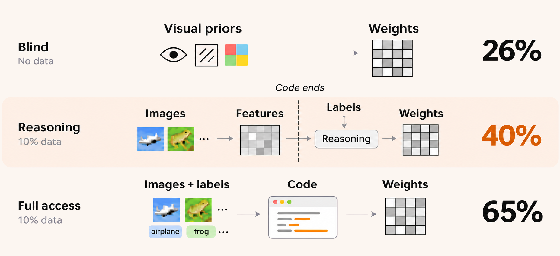
We took part in Ricursive Intelligence's hackathon recently and decided to play around with the shiny new paradigm weight space programming. The core idea is whether or not a language model can write the weights of a neural network instead of training it.
We tasked three models: open-weight Ripple 65B, Claude Opus 5.5, and GPT 6.1 Sol to write weights for a zero-initialized CIFAR-10 ResNet-18 model. We wanted to see how far we can take in-context reasoning about an image dataset with no explicit optimization methods.
Three Ways to Program Weights
There isn't really a universally agreed-upon definition of weight space programming, and it has been interpreted by the community in various ways. We present three different settings, in increasing order of the agent's access and liberty regarding data and tool calls.
We always restrict access to the filesystem and web search in our sandboxed harness. The agent returns its diff to ResNet-18's weights. For conciseness, we summarize the various tools the model has access to in a few pseudo-code function calls:
data(): Access 10% of the training set images. Returns them as a file containing numbers.labels(): Access 10% of the training set labels. Returns them as a file containing integer labels.tools(): Code execution and shell commands. We restrict the model to not use any gradient based fitting methods, and this is carefully audited in all of the implementations.predict(): Use the current ResNet-18 weight diff to run a forward pass on the data. The agent can selectively look at activations at different stages of the model.evaluate(): Use the current ResNet-18 weight diff to evaluate on the 10% training split. It returns the accuracy on the split.submit(): Submit the current weight diff. This ends the interaction.
On top of this set, we divide the experiment into three settings:
| Paradigm | data() | labels() | tools() | Where labels meet data |
|---|---|---|---|---|
| Blind | 🚫 | 🚫 | ✅ | Nowhere (no data) |
| Reasoning 10% | ✅ | In Phase 2 | In Phase 1 | In the agent's context |
| Full access 10% | ✅ | ✅ | ✅ | In code |
Reasoned 10% runs in two phases. In phase 1, the agent can run code on the 4,500 unlabeled images. It then calls end_tools(), which disables code for the rest of the run, and only after that can it request labels. Any fitting of labels to features has to happen in its reasoning.

The two phases for the reasoning 10% regime
We believe this regime is the most interesting, and closest to what we believe weight space programming should mean. The agent can preprocess the input images in whatever way it wants using python / tool calls; but any "fitting" i.e. interaction between labels and features should purely happen in the agent's reasoning context, not via code execution.
In an ideal world, the blind regime would work, as the model could simply reason about the task and write down a working set of weights. It also serves as a useful baseline to check whether the model might have memorized CIFAR-10-specific weights or solutions during pretraining. The full access regime can be seen as letting the model define an "update function" after seeing the data (without gradients ofc) -- i.e. the model acts as the optimizer.
Results
Even without access to CIFAR-10 data, models reached roughly 25% accuracy, well above the 10% chance baseline. More interestingly, Opus reached 40.5% with label-dependent fitting performed entirely in its reasoning context, compared to 65% when that fitting was allowed in code.
| Paradigm | Ripple 65B | GPT 6.1 Sol | Claude Opus 5.5 |
|---|---|---|---|
| Blind | - | 25% | 26% |
| Reasoning 10% | 16% | 29% | 40% |
| Full access 10% | 42% | 62% | 65% |
What the Agents Tried
Full access (10% data)
In this setting, the general behaviour we observed is for the model to loop between engineering features, then updating some weights using closed-form regression/nearest-neighbour type methods by looking at the labels. Effectively, the model acted as its own optimizer without using gradient descent. We see some classic machine learning algorithms showing up in this process - Ripple regularizes its ridge fit, and implements cross validation on the small dataset that it has access to. It also tries to augment the limited data at hand to get a better fit.
Reasoning (10% data)
Early Experiments
In an earlier version of harness where we exposed confusion matrices in evaluate(), Sol recovered the label statistics and fit a classifier in code, reaching 25.53% test accuracy without calling labels().
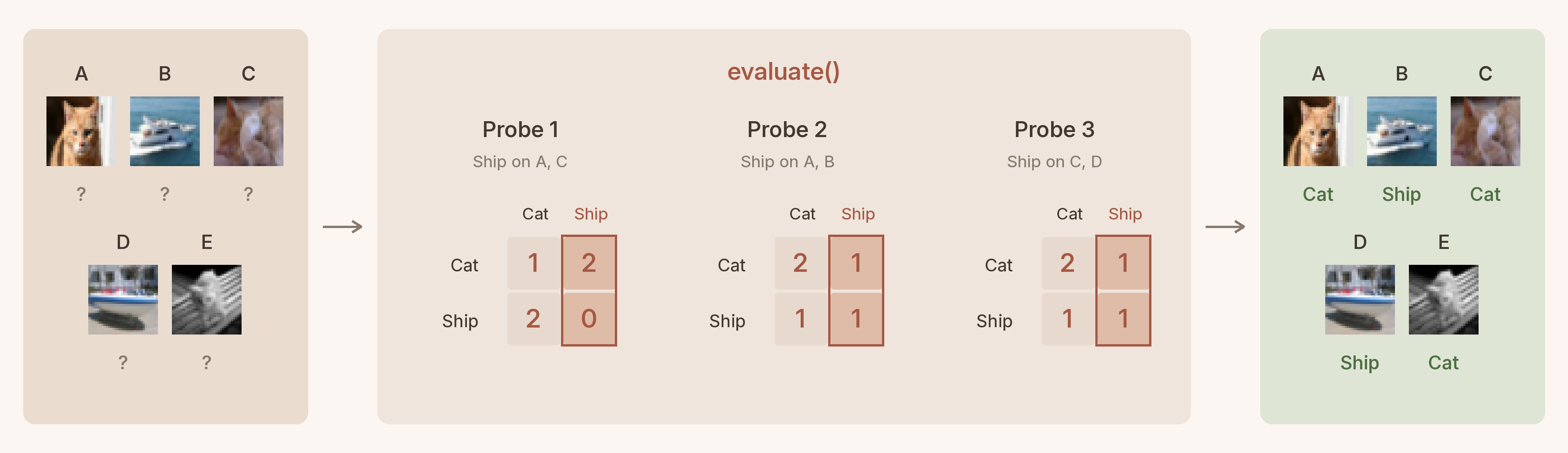
Scaled-down illustrative example of label recovery
With 1% of the data and a text-only interface (we didn't enable the vision encoder), Opus rendered images as ASCII brightness patterns with letters for colors, then tried to recognize the objects:
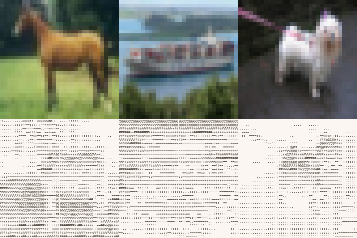
Images and their brightness ASCII patterns
Discovering Semantic Features
Sol’s 10% reasoned run split those steps across the phase boundary. In phase one (where it could compute but couldn’t see labels), it built 40 cluster-derived features and saved the images that activated each one most strongly. In phase two, code was permanently disabled, but labels became available. One feature’s top 20 images included 15 frogs, a strong clue about which output that feature should feed! Sol translated those associations into output weights itself, then adjusted them using accuracy-only feedback.
Constructing a Classifier by Hand
Opus treated the two phases as a pipeline: code turns the unlabeled images into readable units, then it learns the label mapping by hand. In phase 1 it built a classic training-free front end: ZCA-whitened patches, clustered with spherical k-means into 63 conv1 filters, with the rest of the network wired so images fall into 120 clusters, each read out as its own channel. After end_tools(), with no code available, it fetched labels for all 4,500 images, tallied each cluster's class counts in its own reasoning, and wrote those counts directly into fc.weight, so each cluster votes for classes in proportion to what it contained. A one-off predict() on 30 images served as a sanity check, and it submitted without ever calling evaluate(). It scored 39.6% on validation and 40.5% on test, against about 10% for the random start.
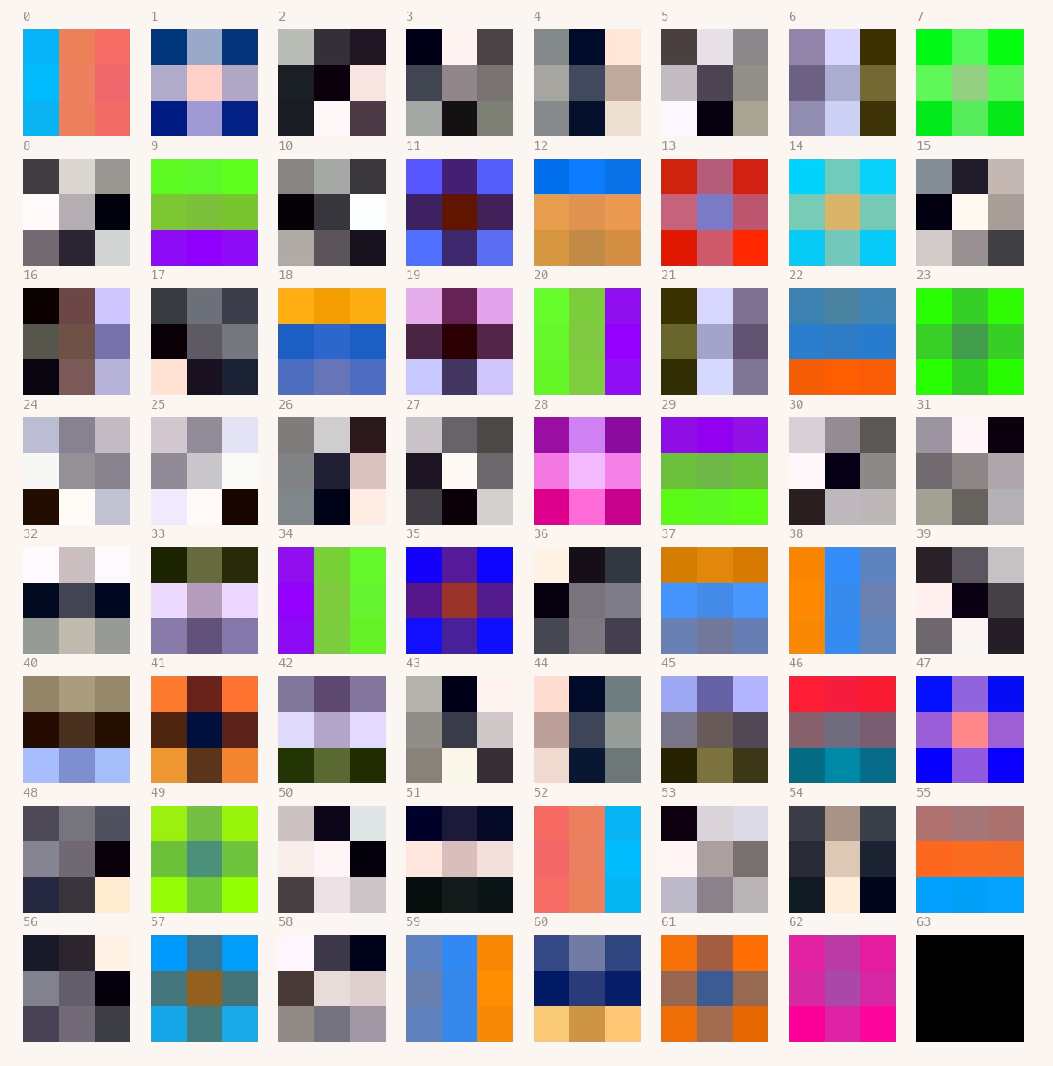
Convolution kernels engineered by Opus based on the k-means
In a trained ResNet, the final linear layer turns the 512 pooled features into ten class scores, and its weights are learned by gradient descent. Opus wrote it from a tally instead. Earlier in the network it had arranged for 120 of those 512 feature channels to act as template detectors: each fires when an image looks like one of 120 groups of training images it had found without labels. Once it was allowed to see labels, it read the class of every image in each group and counted them. Those counts became the weights: the weight from detector to class is simply , the number of class- images in group . A new image 's score for a class is therefore a vote:
where is how strongly detector fires. For example, an image's score for "cat" sums the cat counts of every detector it activates, and the class with the most votes wins.
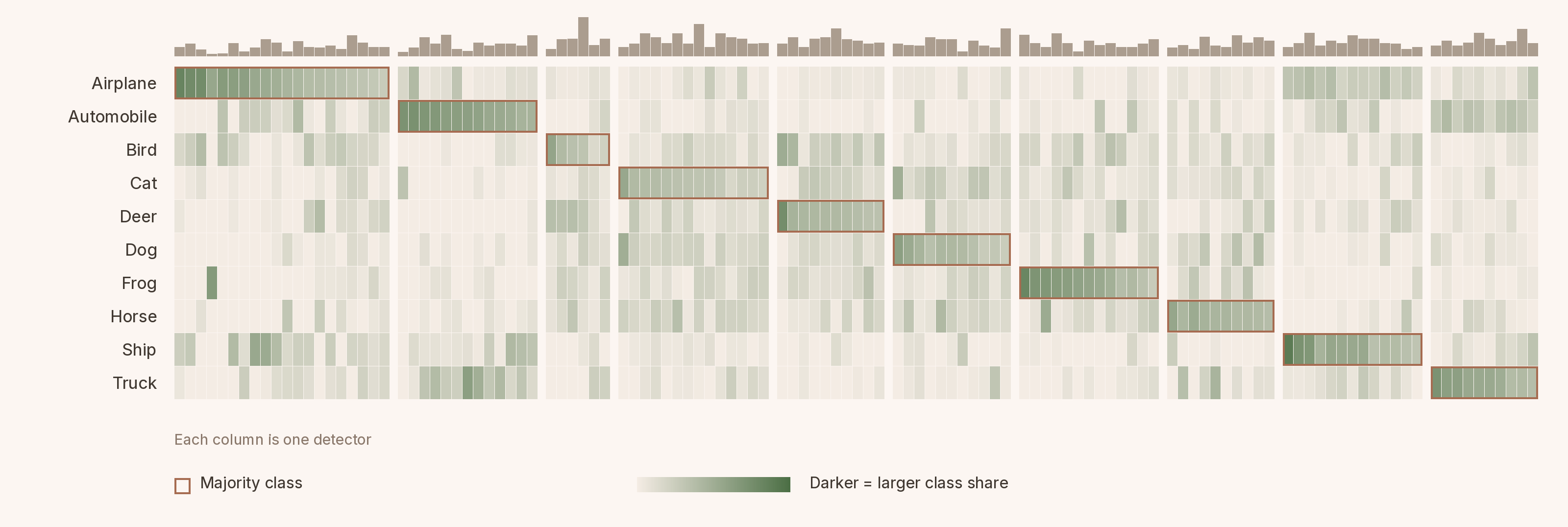
Count-based FC layer: 120 channels grouped by majority class. Easily confused classes, like airplanes and ships (both on blue backgrounds), vote for each other.
Blind
Inventing Training Data
In the blind setting, the models had no data to work from. We ran our harness on GPT 6 Astra, and it responded by writing its own dataset. It drew tiny cars with wheels and windows, deer with antlers, cats with pointed ears, and ships with sails, then added noise, blur, and variations in lighting. It generated 8,000 of these images and used them to fit a classifier. Ripple did the same, but its images looked (slightly) more childish..
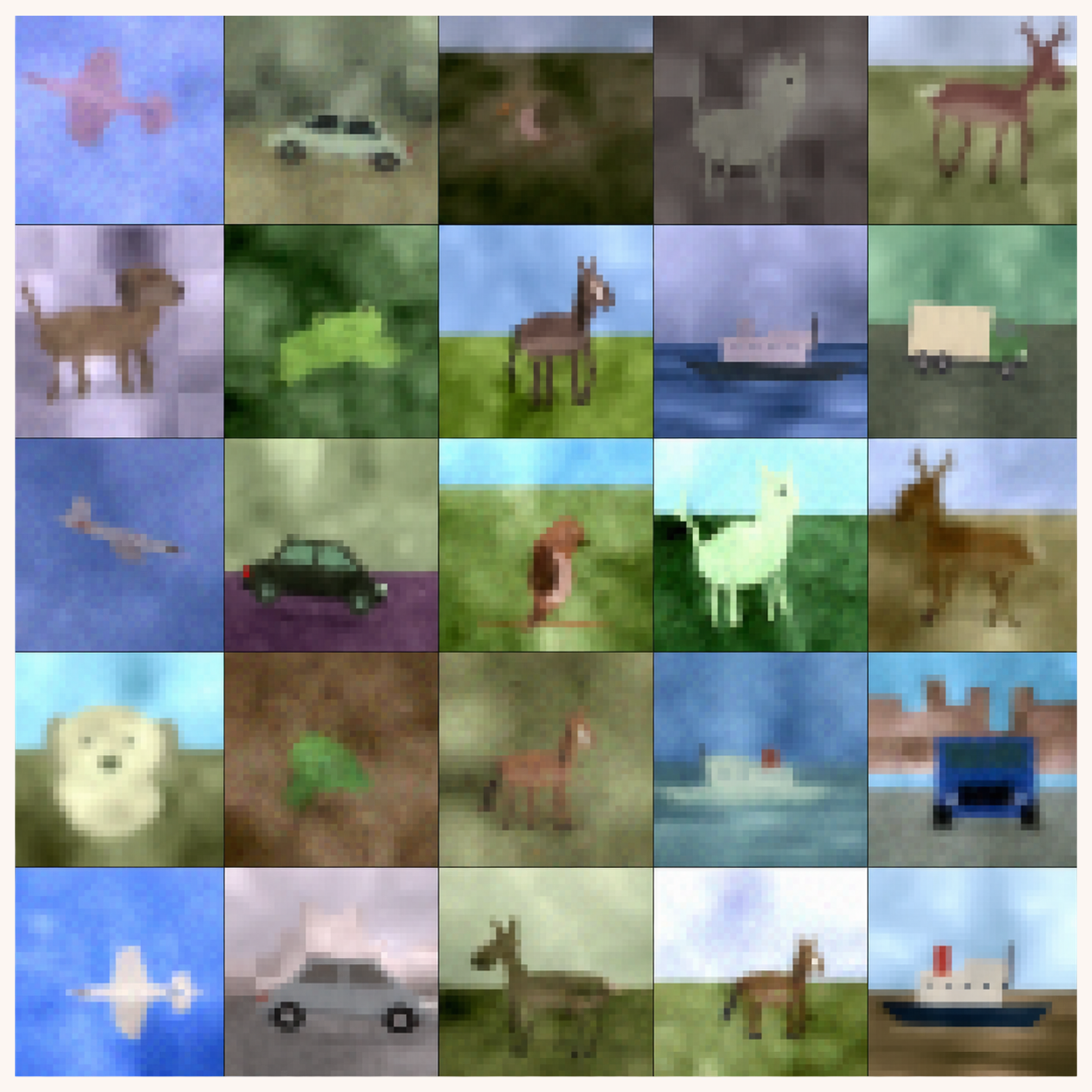
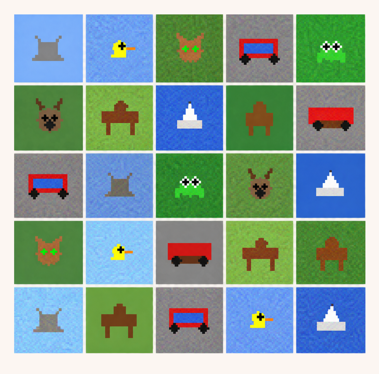
Synthetic training images generated in the blind setting. Left: GPT 6 Astra. Right: Ripple.
Hardcoding Visual Rules
Opus 5.5 took a more direct approach here: it built color and edge detectors into the network and manually connected them to the output classes. Blue and bright counted toward airplane; green counted against it. It also modified the network’s internal paths so those handcrafted features could reach the classifier. Here, you could read the classification rules directly out of the weights it wrote.
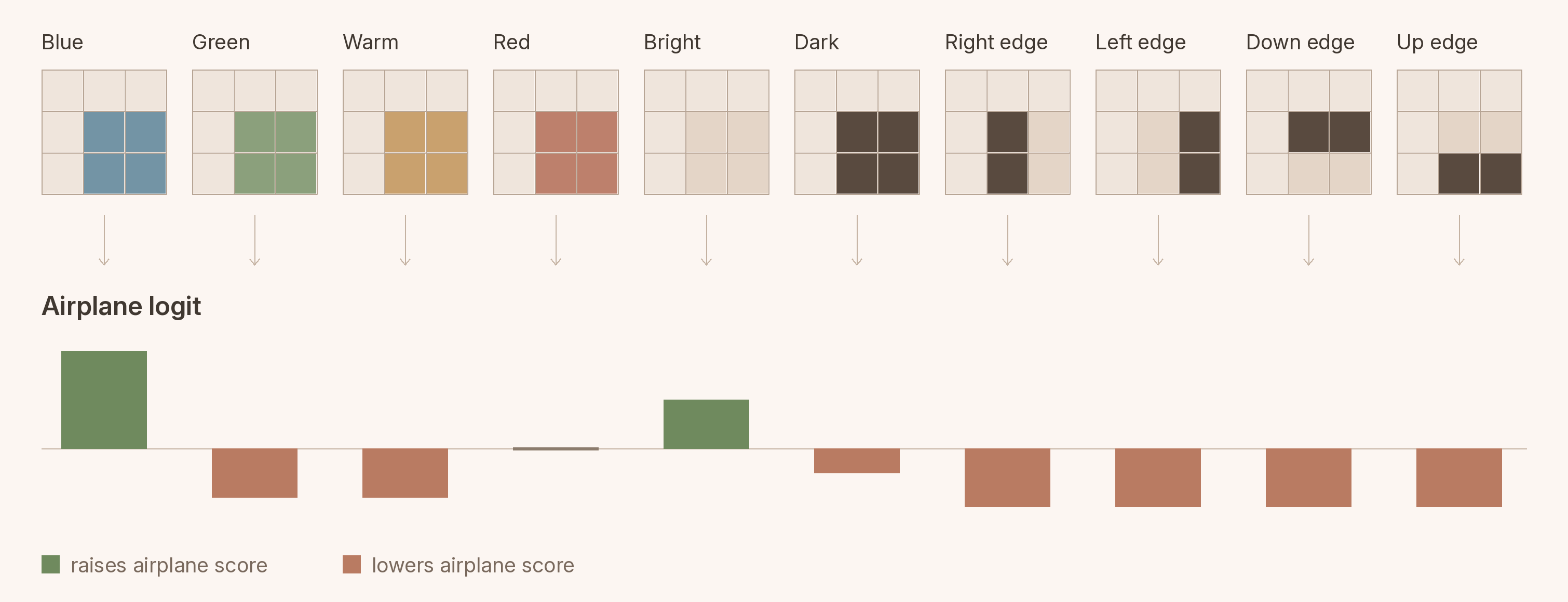
Opus's hand-written color and edge detectors wired to the airplane output
Closing Thoughts
Our favourite part was seeing the strange ways the models approached the problem: engineering features, fitting classifiers with classical methods, constructing synthetic datasets, and writing recognizable classification rules directly into the weights.
The reasoning-only setting felt the most interesting -- Opus managed to construct a useful visual representation without labels, then turn label statistics into a working classifier entirely through in-context reasoning. We're curious how far this can go with better representations (maybe post-training?), larger reasoning budgets, and architectures that are easier to program directly.
If you're interested in looking at the harness, all of the code is available on GitHub!